Analysing the Effect of Trade Shocks on UK Food Trade

undefined

Executive Summary

This report investigates the impact of trade shocks on the United Kingdom’s (UK) food and feed commodity imports, focusing specifically on disruptions caused by weather events and Free Trade Agreements (FTAs). Conducted in partnership with the Food Standards Agency (FSA), the research aims to provide insights into how trade disruptions affect the trade volume of food and feed commodities from partnering countries, employing advanced statistical time series models.

The primary objectives of this study are to identify trade shocks caused by FTAs and weather events, quantify their impacts on UK import volumes, and offer recommendations for future analyses using statistical models. This study employs Interrupted Time Series (ITS) analysis, selected for its effectiveness in assessing the impact of time-specific interventions on trends over time. A key advantage of ITS is its simplicity, as it requires only one type of data – in this case, trade volume data – to perform the analysis. This simplicity allows the methodology to be generalised and applied to various types of trade disruptions, such as FTAs and weather events.

Additionally, the Seasonal Autoregressive Integrated Moving Average (SARIMA) model is utilised due to its effectiveness in capturing complex patterns that repeat over intervals, such as seasonal effects, while also addressing autocorrelation within the data. By incorporating SARIMA, the analysis ensures that the inherent seasonality and temporal dependencies in trade data are accurately modelled, leading to more reliable and robust estimates of the impact of trade shocks.

The models developed in this study focus on four key trade datasets: Ukraine’s trade data, considering the UK–Ukraine FTA and the Russia–Ukraine conflict; Canada’s trade data, considering the UK–Canada FTA; Spain’s trade data, considering the droughts in 2017–2018; and Brazil’s trade data, considering the droughts in 2020–2021. The findings reveal that while the UK–Ukraine FTA did not significantly affect trade volumes, the conflict between Russia and Ukraine has led to a statistically significant decrease in trade. Similarly, the UK–Canada FTA showed no significant impact on trade volumes, although exploratory analysis through visual inspection suggests otherwise.

The study also highlights the disruptions in agricultural trade caused by the droughts in Spain and Brazil, with a more pronounced impact observed in Brazil, where beef exports to the UK were significantly reduced.

Based on these findings, several recommendations are proposed. Expanding the historical scope of trade data is crucial for improving the accuracy and reliability of future analyses. Testing the ITS methodology on different trade datasets is also recommended to assess its robustness and applicability across various contexts. Additionally, standardising the criteria for defining and identifying trade disruptions ensures the consistency and comparability of future studies. From a policy perspective, the significant impact of geopolitical events, such as the Russia–Ukraine conflict, highlights the need for robust contingency plans, strategies to diversify trade partnerships, and efforts to strengthen domestic production capabilities.

In conclusion, this study provides a comprehensive assessment of the impact of FTAs and weather events on the UK’s food and feed imports. The use of ITS and SARIMA models offers valuable insights for policymakers, helping them to develop strategies that mitigate the adverse effects of trade shocks and ensure greater stability and resilience in the UK’s food supply chain.

1. Introduction

1.1. Overview

Food security is a cornerstone of global well-being and sustainable development. The term “food security” is defined as a condition whereby every person has sufficient access, both physically and economically, to safe and nutritious food in order to lead a healthy and active life. According to the World Bank (The World Bank, 2024), four essential conditions must be met to achieve food security:

1. Availability: ensuring enough food is produced and available to meet the dietary needs of all people.

2. Accessibility: providing sufficient economic and physical access to food for everyone.

3. Utilisation: ensuring that the food consumed is safe and provides the necessary nutrients for a healthy life.

4. Stability: maintaining consistent access to food, even in the face of adverse conditions such as weather events and political conflicts.

The importance of achieving food security cannot be overstated because it is part of the fundamental aspect of the United Nations’ Sustainable Development Goals (SDGs), particularly Goal 2: Zero Hunger. This goal aims to end hunger, achieve food security and good nutrition by 2030 by using a comprehensive range of strategies from enhancing domestic agricultural practices to fostering international cooperation (United Nations, 2024). Consequently, food security has become a paramount concern among global leaders.

Achieving food security has become increasingly challenging from multiple perspectives, particularly from both the supply and the demand sides.

On the supply side, factors driving food production include regulatory frameworks, agricultural investments and environmental health (Pinstrup-Andersen & Pandya-Lorch, 1995). Regulatory frameworks range from laws governing agricultural practices to international trade regulations. Agricultural investments involve providing the resources needed to ensure continuous agricultural advancement and growth. Environmental health includes implementing necessary measures to prevent environmental degradation.

On the demand side, factors influencing food consumption encompass income levels, food prices and consumption preferences (Pinstrup-Andersen & Pandya-Lorch, 1995). These demand-side drivers determine the purchasing power of individuals and the types of food they prioritise, which in turn affects their food security.

The United Kingdom (UK), with a population of nearly 68 million, relies on both domestic production and imports to meet its food consumption needs (Office for National Statistics, 2024). As of 2020, it sourced 46% of its food through imports (Department for Envionment, Food and Rural Affairs, 2023). However, due to its heavy reliance on imports, the flow of food supplies is vulnerable to disruptions caused by trade shocks, which can result in unexpected changes in trade patterns. For instance, the conflict that began between Russia and Ukraine in 2022 had a significant impact on Ukraine’s agricultural production: during the three years preceding the war (Janzen & Zulauf, 2023), Ukraine accounted for 15% of the global corn trade and 10% of the global wheat trade. Concurrently, Ukraine’s cereal exports to the UK declined by nearly 72% in 2022 (Trading Economics, 2024). This highlights the importance of understanding the implications of current disruptions on food and feed imports into the UK.

In response to such challenges, this thesis examines the trade shocks occurring among the UK’s trade partners and analyses the implications of these trade shocks on the UK’s imports. By examining historical data and trends, it aims to provide quantifiable insights into how specific trade shocks can have an impact on food trade volumes. Consequently, this analysis is expected to enhance the understanding of food and feed trade, and also better equip policymakers to address relevant trade shocks in the future.

1.2. Trade shock

To ensure consistency throughout this report, I shall define the term “trade shock”: it is characterised by significant changes, either positive or negative, in trade flows, resulting in abrupt shifts in trade volumes and/or prices. Various factors can cause trade shocks, such as:

1. Geopolitical events: the recent Russia–Ukraine conflict has caused substantial trade disruptions in commodities, including agricultural products (Cevik, 2023).

2. Weather events: the hurricane Florence in North Carolina in September 2018 resulted in more than $1.1 billion in damages to crops and livestock (AgAmerica, 2019).

3. Regulatory changes: the European Union (EU)–South Korea Free Trade Agreement (FTA) illustrates how FTAs can induce positive trade shocks by enhancing market access and reducing trade barriers (Jung, 2023).

4. Pandemics and health crises: The COVID-19 pandemic, led to sudden and severe disruptions in trade flows due to labour shortages, logistical challenges, consumer demand, and challenges in production and distribution (Barman, Das, & De, 2021).

Given the frequent occurrence of trade shocks, this thesis will focus on understanding the relationship between trade shocks and the volume of food and feed commodity imports to the UK. Specifically, the scope of trade shocks is limited to those caused by weather events and Free Trade Agreements (FTAs), as discussed with the Food Standards Agency (FSA). This research is motivated by and conducted in partnership with the FSA.

1.3. About the Food Standards Agency

The FSA is an independent government department in the UK, established in 2000. Its primary responsibility is to protect public health in relation to food and to ensure that food is safe, accurately described and healthy to consume. The FSA operates across England, Wales, and Northern Ireland.

Some of the key functions of the FSA include the following:

1. Food safety and hygiene: setting and enforcing standards to ensure that all food produced or sold in the UK is safe and hygienic.

2. Labelling and consumer information: ensuring that food labels are accurate and informative, covering nutritional information, allergen warnings, and country of origin; creating resources and campaigns to educate consumers about food safety and nutrition.

3. Fraud prevention and authenticity: monitoring and enforcing against fraudulent activities to tackle food fraud and ensure authenticity.

4. Research, policy, and incident response: conducting scientific research to inform the best food safety policies and practices and managing food safety incidents.

5. Trade monitoring: monitoring food trade between the UK and its global partners to anticipate food hazards, and to help analyse policy decisions.

The FSA faces a challenge in both anticipating the current trade shocks faced by its importing countries and understanding their impact on the volume of imports. The agency requires assistance in determining whether these trade shocks truly affect the volume of food trade from specific importing countries. The scope of trade shocks discussed is limited to those caused by weather events and FTAs due to their frequency of occurrence and relevance to the FSA’s interests. This report aims to provide a guideline for the FSA when facing similar trade shocks in the future.

1.4. Objectives of the research

The objectives of the research are as to:

• identify shocks caused by weather events and FTA, and their relationship with the volume of imports to the UK;

• analyse the impact of these trade shocks on the UK’s food and feed commodity imports;

• provide a methodology to quantify trade shocks in trade volumes; and

• provide the FSA with recommendations for effectively analysing future trade shocks using statistical models.

1.5. Tools

The tools used throughout this research are the R programming language and Microsoft Office Excel. Details on the coding packages used and their implementation are elaborated in Section 3.5.

1.6. Structure of the report

This report consists of the following five chapters:

• Chapter 2 provides an overview of related works relevant to this study and evaluates the gaps in the literature that motivate this research.

• Chapter 3 elaborates on the methodology used in this study, from data collection through to software implementation.

• Chapter 4 discusses the results of the models, incorporating both exploratory analysis, which provides an initial visual inspection, and statistical analysis, which quantifies the insights derived from the exploratory analysis.

• Chapter 5 concludes the study and provides recommendations for future work in this area.

Appendix A contains a step-by-step guide to model development in R for UK-Ukraine trade data.

2. Literature Review

This chapter aims to contextualise the research and is divided into four sections. The first section sets the context behind free trade agreements (FTAs) and weather events to ensure that readers are in agreement about these terms. The second section introduces relevant work in this area. The third section reviews the methodologies used in related studies and discusses the interrupted time series methodology being considered for this study. The final section identifies research gaps as part of considerations for this study.

2.1. Context and background

Understanding the foundational concepts central to this research is crucial. This section delves into two primary areas: FTAs and weather events. By providing a detailed overview of these topics, the aim is to ensure a comprehensive grasp of the key terms and contexts necessary for the subsequent analyses and findings.

2.1.1. Free Trade Agreement

An FTA is an arrangement between two or more countries that establishes specific obligations related to trade in goods and services, investor protections, and intellectual property rights (International Trade Administration, 2024). Its primary objective is to reduce barriers to trade, thereby making it easier and less costly for countries to exchange goods and services.

Following Brexit, the United Kingdom (UK) was compelled to negotiate its own trade agreements to replace those previously held through European Union (EU) membership. This has led to the establishment of more than 70 new FTAs since 2020, aimed at ensuring continuity in trade and expanding the UK’s trade network independently of the EU, with several others still under negotiation (Department for Business and Trade & Department for International Trade, 2020). However, there are several FTA implications and challenges that need to be addressed:

1. Before Brexit: the UK was part of the EU and benefited from the trade agreements established by the EU. These agreements facilitated seamless trade between member countries and with other global partners, ensured minimal trade barriers and standardised regulations.

2. After Brexit: the UK had to renegotiate many of its trade agreements to ensure continued access to global markets. This period saw the establishment of new FTAs with countries outside the EU and the modification of existing agreements to reflect the UK’s new status as an independent trading nation. This transition period posed significant challenges, including ensuring regulatory alignment, managing tariffs, and addressing non-tariff barriers (Institute for Government, 2023).

A notable example of an FTA is the EU–Canada Comprehensive Economic and Trade Agreement (CETA). This trade agreement was signed on 30 October 2016 and entered into force provisionally on 21 September 2017. It aimed to remove 98% of the tariffs between the EU and Canada and to address non-tariff barriers to facilitate trade (European Commission, 2024).

Post-Brexit, the UK and Canada signed the UK–Canada Trade Continuity Agreement in December 2020, which entered into force on 1 April 2021. This agreement ensures seamless trade between the UK and Canada, largely replicating the terms of CETA and maintaining tariff-free trade on 98% of goods traded between the two nations. The transition was seamless because this agreement preserved the benefits of CETA, allowing businesses to continue trading under the same terms without interruption (UK Government, 2020). This continuity was crucial in maintaining stable trade relations and providing certainty for businesses operating between the two countries.

2.1.2. Weather events

Weather events are significant meteorological phenomena that can have a substantial impact on the environment and human activities. According to the Met Office, extreme weather events such as heatwaves, heavy rainfall and storms are increasingly linked to climate change, with global warming intensifying these occurrences (Met Office, 2024). Human activities, particularly greenhouse gas emissions, have heightened the frequency and severity of these events (Department for Energy Security and Net Zero, 2014).

In the context of trade shocks, it is important to understand the difference between weather events and climate change. Climate change involves long-term shifts in temperature and weather patterns due to activities like greenhouse gas emissions and deforestation (IPCC, 2013). These shifts result in extreme weather events, such as prolonged droughts, intensified hurricanes and rising sea levels, which are direct consequences of climate change. Higher global temperatures contribute to polar ice melting, leading to higher sea levels and coastal erosion, while altered precipitation patterns cause severe droughts and flooding. These changes have a significant impact on agriculture, water resources and human settlements. Understanding these connections is crucial for assessing their impact on trade and food security.

Notable examples of extreme weather events influenced by climate change include the following:

1. Hurricanes: the 2020 Atlantic hurricane season was the most active on record, with 30 named storms, including hurricanes Laura and Delta, causing widespread damage and significant economic losses. This unprecedented activity was linked to climate change because warmer-than-average sea surface temperatures and reduced vertical wind shear, both influenced by global warming, provided more energy for storm formation and intensification (National Oceanic and Atmospheric Administration, 2020).

2. Heatwaves: the 2019 record temperatures in South Africa set new extreme heat records across the country, leading to severe impacts on public health and agriculture. The extreme heat contributed to a situation whereby a record 45 million people faced food shortages (Heiberg, 2019).

3. Floods: the 2016 flooding in France and Germany, caused by extreme rainfall, devastated parts of both countries. These floods were exacerbated by global warming, which has increased the frequency and intensity of extreme weather events, thereby contributing to higher rainfall levels and more severe flooding conditions (Climate Signals, 2016).

2.2. Related works

Relevant work in this area is quite limited, but several key studies have made significant contributions to our understanding of the impact of FTAs and weather events on food trade and security.

Studies on FTAs address various perspectives. Kiyota and Stern (Kiyota & Stern, 2007) analyses the potential economic impacts of signing an FTA between the Republic of Korea and the United States (US), with the agreement still under negotiation during the time of this study. With the objective of promoting mutual benefits for both parties through the agreement, the study concludes that the Korea–US FTA would yield substantial economic benefits for both countries, enhancing bilateral trade and investment relations while promoting broader economic integration and cooperation in the Asia–Pacific region.

Another interesting perspective is seen in (Khati & Kim, 2023), where the report intends to review the impact of the current FTA between India and the Association of Southeast Asian Nations (ASEAN), and to provide insights into future improvements to make the partnership more beneficial. By utilising 2000–2019 panel data, and noting that the ASEAN-India Free Trade Agreement (AIFTA) was signed in 2009 and came into effect in 2010, the study concludes that, while AIFTA has increased trade between India and ASEAN, it has not significantly boosted India’s exports to the region, partly due to rising Non-Tariff Measures (NTMs).

At the same time, (Cowling et al., 2020) is a comparative study that aims to analyse the impact of US FTAs, following their implementation, on the sales of processed foods in partner countries following the implementation of US FTAs. The research concludes that joining US FTAs is associated with increased sales of highly processed foods that have negative implications for public health. Specifically, it highlights how the rise in consumption of these foods contributes to higher rates of non-communicable illnesses, such as obesity and cardiovascular diseases, in the affected countries.

Three reports on FTAs collectively illustrate varied approaches to assessing their impacts. Kiyota and Stern’s prospective analysis of the Korea–US FTA explores the potential economic benefits before the agreement’s signing, emphasising regional integration (Kiyota & Stern, 2007). In contrast, Khati and Kim’s retrospective evaluation of the India–ASEAN FTA examines its mixed results post-implementation, highlighting the issue of NTMs (Khati & Kim, 2023). Meanwhile, Cowling et al.'s comparative study focuses on public health, revealing increased sales of highly processed foods in countries with US FTAs (Cowling et al., 2020). These differing perspectives underscore the multifaceted effects of FTAs, informing the broader discourse on their economic and health implications and providing better context for the angle taken in this study.

Researches specifically assessing extreme weather events’ impacts on food commodities are lacking, while more focus is given to the impact of climate change on food production using panel data analysis. For instance, (Emediegwu & Ubabukoh, 2023) examines the relationship between weather changes and global livestock production, particularly beef. Using cattle production, weather and climate change prediction data across 187 countries, and using an econometric approach, the research discusses how temperature and precipitation changes have an impact on global beef production. It concludes that climate change has a significant effect on global livestock production, with more severe effects in tropical, poor, and agriculture-dependent regions.

Powell and Reinhard (Powell & Reinhard, 2016) aims to quantify the effects of extreme weather events on winter wheat yields in the Netherlands. The paper uses weather variables, establishing a link between climate change and the frequency of extreme weather events by analysing long-term weather data. It demonstrates that climate trends are linked to the frequency of extreme weather events and concludes that the increasing frequency of these events will continue to adversely affect wheat yields.

Another paper (Kapsambelis et al., 2022) is taking a similar angle as the previous literature in modelling the impact of extreme droughts on agricultural yields in France under current and future climate conditions. While the study focuses on drought, it links the frequency of extreme droughts to yield loss by analysing meteorological variables such as precipitation, temperature and evapotranspiration. These variables are used to determine the occurrence and intensity of droughts, which are then correlated with yield data for grasslands and cereals to assess their impact. The study concludes that the increasing frequency of extreme droughts due to climate change will have a significant impact on agricultural yields.

Collectively, these papers (Kapsambelis et al., 2022; Powell & Reinhard, 2016) underscore the relationship between extreme weather events and crop yields by demonstrating that climate-related variables directly influence the frequency and intensity of such events. Integrating econometric analysis with detailed climatic data provides a robust framework for predicting and managing future risks to agricultural productivity. As the frequency of extreme weather events rises, understanding their specific impacts on different types of crops and regions becomes crucial for formulating effective policies and interventions aimed at ensuring sustainable food production in a changing global climate.

Although the analytical approaches taken in studying FTAs and weather events are quite different, the overarching objective of all the studies discussed here is to assess their respective impacts on trade and agricultural production. The FTA studies, such as (Kiyota & Stern, 2007), (Khati & Kim, 2023) and (Cowling et al., 2020), primarily focus on economic assessments, examining how trade policies influence market dynamics, trade volumes, and public health outcomes. In contrast, the weather event studies (Powell & Reinhard, 2016) and (Kapsambelis et al., 2022) employ meteorological, weather and agricultural data to explore the direct impacts of weather events on crop yields. Despite these methodological differences, both sets of studies share a common goal: to provide valuable insights into how external factors – be they policy changes or environmental shifts – affect critical aspects of food security and economic stability. Through thorough analyses, policymakers can better develop strategies to mitigate negative outcomes and enhance resilience in agricultural and trade systems.

2.3. Methodological approaches

This section delves into the various methodological approaches employed in related works to provide a clearer understanding of the techniques used and their implications. The discussion is divided into two main subsections: the first explores the methodologies adopted in studies related to FTAs and weather events, while the second focuses on the Interrupted Time Series (ITS) design. ITS is proposed for this study due to its ability to analyse the impacts of time-specific interventions, specifically FTAs and weather events, on trends over time.

2.3.1. Methodology among related works

The methodologies in related works vary significantly, both between studies on FTAs and climate variability and within each individual topic. This section delves into the methods and implications of each discussed work to provide clearer context.

Kiyota and Stern (Kiyota & Stern, 2007) uses the Michigan Model of World Production and Trade, a comprehensive computational general equilibrium (CGE) model that covers 27 economic sectors in 30 countries. It accounts for imperfect competition, increasing returns to scale and monopolistic competition. The analysis simulates the removal of trade barriers, conducting both static and dynamic analyses to consider long-term capital formation and foreign direct investment adjustments. Extensive data from the Global Trade Analysis Project database is used to model economic adjustments and sectoral interdependencies, making the analysis thorough yet complex.

Khati and Kim (Khati & Kim, 2023) employs a gravity model to study the impact of AIFTA on India’s goods exports. This reliable model examines trade flows based on economic size and distance where trade volume is proportional to gross domestic product (GDP) and inversely proportional to distance (Chaney, 2013). The research uses panel data from 2000 to 2019, encompassing pre- and post-AIFTA periods, with variables such as GDP, common language, trade openness and NTMs. Using a random effects model, it controls for unobservable heterogeneity, offering a comprehensive view of AIFTA’s trade dynamics and policy implications.

Cowling et al. (Cowling et al., 2020) applies a comparative interrupted time-series (CITS) analysis to assess the impact of US FTAs on processed food sales in partner countries. CITS, a quasi-experimental design, evaluates effects when randomised controlled trials are infeasible (Cowling et al., 2020). This paper uses annual data from 2002 to 2016, comparing processed food sales trends between countries that joined US FTAs (the treatment group) and those that did not (the control group). Although CITS is a more straightforward model compared with the CGE and gravity models, it effectively controls for variables like GDP per capita, urbanisation rate and female labour force participation rate, making it an interesting approach with which to isolate the effect of FTAs.

While researches on the impact of FTAs on trade employ a variety of complex economic models, researches on weather events also provide interesting insights using diverse methodologies. Some researches use straightforward regression analysis while others use specialised climatic models.

The papers (Powell & Reinhard, 2016) and (Kapsambelis et al., 2022) integrate meteorological data with agricultural outputs to assess climatic impacts on crop yields. Powell and Reinhard (Powell & Reinhard, 2016) use a fixed-effects panel regression model to control for time-invariant characteristics across farms. This method isolates the impact of extreme temperature and precipitation events on winter wheat yields in the Netherlands over a 12-year period, incorporating economic variables such as pesticides, fertilisers, labour and capital to ensure precise insights.

Similarly, Kapsambelis et al. (Kapsambelis et al., 2022) employ the Drought Occurrence and Weighted Key Index (DOWKI) and the Action de Recherche Petite Echelle Grande Echelle (ARPEGE)-Climate Model. The DOWKI quantifies drought frequency and intensity, while the ARPEGE-Climate Model projects future climatic conditions. This combination provides a robust framework for assessing drought impacts by correlating climatic indices with yield data. Integrating data on precipitation, temperature and evapotranspiration with yield data for grasslands and cereals in France, the article projects the impacts of future drought various climate scenarios.

2.3.2. Interrupted Time Series

Interrupted Time Series (ITS) is a quasi-experimental design that evaluates the impact of an intervention or event by comparing the trends in the outcome variable before and after the intervention (Turner et al., 2021). This approach allows for a detailed assessment of how these shocks disrupt normal trade patterns and it helps to isolate their specific impacts from other underlying trends.

ITS design is particularly useful in scenarios where randomised controlled trials are not feasible, and it has been widely used in various fields including public health, economics and the social sciences. By analysing a single series of data points over time, ITS can control for autocorrelation and other confounding factors that might influence the outcome variable, providing robust insights into the causal effects of interventions (Turner et al., 2021).

A key feature of ITS is the ability to visualise and statistically analyse changes in level and trend before and after the intervention using segmented regression analysis. This method estimates the intervention effect while accounting for underlying trends and seasonality (Wagner et al., 2002). It distinguishes between immediate and gradual changes postintervention, which is crucial for understanding the dynamics of trade shocks. This methodological rigour ensures that ITS remains a robust tool for causal inference in various applied research contexts.

To determine whether ITS is suitable for a specific issue or project, several key checkpoints should be considered (Turner et al., 2021):

1. Availability of data: sufficient data points must be available both before and after the intervention, ensuring the reliability of the analysis. Wagner et al. (Wagner et al., 2002) recommend having at least 12 data points each, both before and after the intervention.

2. Timing of intervention: the exact timing of the intervention must be clearly defined in order to identify accurately its impact on the outcome variable.

3. Presence of clear trends: there should be discernible trends in the data before and after the intervention for the effective application of segmented regression analysis.

4. Lack of other simultaneous interventions: the presence of other interventions or events occurring at the same time can confound the results, making it difficult to isolate the impact of the intervention under study.

5. Handling of autocorrelation: ITS must be able to control for autocorrelation in the data to avoid biased estimates of the intervention effect.

Some researchers have employed ITS to evaluate the impacts of various interventions. For example, Lopez Bernal et al. (Bernal et al., 2017) used ITS to examine the effect of public smoking bans on hospital admissions for cardiovascular and respiratory conditions across multiple countries, and demonstrated significant reductions in admissions post- implementation. Similarly, a study by Suah (Suah, 2023) used ITS to evaluate the impact of COVID-19 cash handouts on daily spending in Malaysia. That research found that the cash handouts led to a positive and significant increase in spending, which dissipated within a month. Another study by Cruz et al. (Cruz et al., 2017) applied ITS to analyse the effectiveness of a new healthcare intervention model on patient satisfaction in hospitals, and this showed notable improvements in patient satisfaction post-intervention. These articles highlight the robustness and versatility of ITS, allowing researchers to draw causal inferences about the effectiveness of various interventions over time.

Questions may arise due to the insufficient cases of ITS specifically addressing the issues to be discussed in this study. However, the methodology’s adaptability to various fields suggests its potential effectiveness in this context. By carefully tailoring the ITS design to account for the unique characteristics of trade data and climate change impacts, this study aims to provide new insights into how such shocks affect trade volumes. The use of ITS in this research will help bridge the gap in existing literature and demonstrate its applicability to trade and climate-related interventions.

2.4. Gaps in the literature

The existing literature has made significant contributions to understanding the economic impacts of FTAs and the agricultural impacts of weather events. However, several gaps persist, which this research aims to address.

Comprehensive analyses exist on the economic impacts of FTAs, such as those in studies (Kiyota & Stern, 2007), (Khati & Kim, 2023) and (Cowling et al., 2020), as well as on the agricultural impacts of weather events, including studies (Powell & Reinhard, 2016) and (Kapsambelis et al., 2022). However, these issues have typically been treated separately, each employing distinct models without considering a unified approach that can address both types of shocks in a coherent framework.

A critical gap is that, while methodological approaches such as panel data analysis and CGE models have been widely used, these models are not easily applicable for the Food Standards Agency (FSA) when assessing whether shocks in partnering countries affect the trade volume to the UK. This difficulty arises because these approaches often require extensive and detailed data, which may not be easily obtainable. For instance, the analysis in (Powell & Reinhard, 2016) requires data from 2002 to 2013 on winter wheat production inputs across 300 farms in the Netherlands, along with weather data including temperature and evapotranspiration. While this results in a robust framework, these models necessitate many variables, adding to the complexity and making them less practical for quick assessments.

Aside from that, while many articles state the causal relationship between a certain weather event and crops, they do not include studies that model the causal relationship in a statistical manner. For instance, an article might state that the production of fruits and vegetables in Spain, in areas similar to Costa Blanca, decreased by 25% due to drought in December 2023, yet there is no statistical model that backs this reasoning. Also, while studies like (Powell & Reinhard, 2016) and (Kapsambelis et al., 2022) address issues on the frequency of extreme weather events and crops, producing these results takes some time, while the FSA needs to act quickly whenever there are trade shocks in order to support policymakers in making decisions to ensure food security in the country.

To address these gaps, this study proposes the use of ITS analysis. ITS is particularly suited for evaluating the impacts of trade shocks from FTAs and climate change, represented by weather events, on trade flows and food security due to a) its ability to handle data with temporal structures, and b) its robustness in distinguishing intervention effects from underlying trends.

Despite the lack of related works employing ITS for this specific case, the methodology fits well for several reasons. ITS is effective in scenarios where randomisation is not feasible, making it ideal for analysing real-world trade data where controlled experiments are impossible. Also, ITS can control for autocorrelation in the data, a common issue in time series analysis, thereby ensuring more reliable results. The ability to handle temporal dependencies and identify causal impacts from interventions further supports its suitability for this study.

By applying ITS, this study aims to provide a detailed assessment of how these shocks disrupt normal trade patterns and isolate their specific impacts from other underlying trends.

Therefore, integrating insights from both FTAs and weather event studies to form a cohesive understanding of their impacts on trade flows and food security is essential. This comprehensive approach, using ITS, can help in developing strategies that are not only theoretically sound but also practically applicable in the context of the UK’s food and feed imports, allowing the UK to be better prepared and more resilient in its actions.

3. Methodology

In this chapter, I propose a comprehensive methodology to address the gaps identified in the literature. The methodology of this study is meticulously designed to evaluate the impact of trade shocks from free trade agreements (FTAs) and weather events on trade flows and food security using Interrupted Time Series (ITS) analysis. The first section elaborates on the data sources and pre-processing required to prepare the data. The second and third sections introduce the ITS design and the Seasonal Autoregressive Integrated Moving Average (SARIMA) model, essential concepts for building the analytical framework. The fourth section discusses the analytical framework necessary to ensure that the model adheres to theoretical assumptions. The final section outlines the software and tools employed.

3.1. Data collection and pre-processing

This section gathers and prepares the necessary data for analysing the impact of FTAs and weather events on trade flows. It is divided into two subsections: data sources and data pre-processing.

3.1.1. Source of data

The data used in the analysis is from public sources and collected by the Food Standards Agency (FSA). The datasets include the following:

1. Food and feed list: available on the FSA website^[1]. This dataset provides an inventory of food and feed products categorised by the following commodity codes and descriptions, including:

   • Commodity code: an 8-digit unique identifier.

   • Description: brief product description.

   • Food: indicates if for food or not.

   • Feed: indicates if for feed or not.

   • Product is of animal origin (POAO) or non-animal origin (FNAO: specifies which.

   • Category: type of food and feed.

2. UK Trade data: sourced from His Majesty’s Revenue and Customs and published on the UK Trade Info website^[2]. This dataset details the importation of food and feed products to the UK from 2014 to 2023, as follows:

   • 2-digit Comcode: the first two digits of the commodity code indicating the broader product category.

   • 2-digit description: description corresponding to the 2-digit Comcode.

   • Commodity code: an 8-digit unique identifier.

   • Port code: code for the port of arrival.

   • Port name: full name of the port.

   • Port type: type of port (airport or seaport).

   • Country code: code representing the origin country.

   • Country name: full name of the origin country.

   • Month: the month and year of import.

   • Value: monetary value of the consignment in British pounds.

   • Weight: weight of the consignment in kilograms.

   • Number of consignments: count of individual consignments.

   • Commodity description: detailed product description, including specific characteristics such as fat content and packaging details.

3. Trade shock data: since the UK trade data is only available from 2014 to 2023, the trade shocks need to be limited to this time frame. Careful consideration is required when choosing the trade shocks, such as:

   a. Rotterdam–Antwerp effect: refers to distortions in trade data caused by goods passing through major ports like Rotterdam and Antwerp before reaching their final destination. These ports serve as major shipment hubs, leading to goods entering the UK being misattributed to these ports. As a result, trade volumes from these ports do not accurately reflect the true origin of the goods, causing inaccuracies in trade data and complicating the analysis of trade flows from the Netherlands and Belgium to the UK (Mion & Aznar, 2023).

   b. Sufficient data points: ensuring enough data points before and after the intervention is crucial for meaningful analysis. While there is no precise number, general recommendations suggest having at least 12 data points each before and after the intervention. This guideline, although not based on strict power estimates, helps in providing robust and reliable results (Wagner et al., 2002).

As such, four shocks were selected for analysis in this study from various sources: two related to FTAs and two to weather events. Details are as follows:

• UK–Ukraine FTA: the UK–Ukraine Free Trade Agreement, replacing the EU-Ukraine FTA due to Brexit, entered into force on 1 January 2021. This agreement replicates the terms of the EU–Ukraine FTA to ensure continuity in trade with no transition period. Therefore, the starting date for the intervention is considered to be the provisional in-force date of the original EU–Ukraine FTA, which is 1 January 2016 (Department for Business and Trade & Department for International Trade and Foreign, Commonwealth & Development Office, 2020). Also, the ongoing Russian–Ukraine conflict on 24 February 2022 has significant implications for trade and economic stability, making it an important factor to consider in the analysis of trade shocks (Walker, 2024).

• UK–Canada FTA: the Canada–UK Trade Continuity Agreement (TCA), replacing the EU–Canada Comprehensive Economic and Trade Agreement (CETA) due to Brexit, entered into force on 1 April 2021. This agreement largely replicates the terms of CETA to ensure continuity in trade without any transition period. Thus, the starting date for the intervention is considered to be the in-force date of the original CETA, which was 21 September 2017 (UK Government, 2020) (Burden, 2020).

• Spain drought: the 2017–2018 drought in Spain, considered the worst in decades, began in mid-2017 and continued through 2018, severely affecting agricultural productivity and water resources. In particular, Castile and Léon, Spain’s largest cereal-growing region, experienced crop losses estimated between 60% and 70%. This period is used as an intervention point due to its substantial impact on the agricultural sector (Sevillano, 2017) (Madrid, 2017).

• Brazil drought: the 2020–2021 drought has been described as the worst in almost a century, particularly in central and southern Brazil. Spanning from approximately September 2020 to June 2021, it marks some of the driest conditions in nearly a century, recording its lowest rainfall in 91 years. This drought led to critically low water levels in major reservoirs, disrupting hydroelectric power generation, and having a severe impact on agricultural production (Grimm et al., 2020) (Patel, 2021).

Also, for each trade shock, the analysis is conducted on the trade volume of specific food and feed commodities imported from the respective partnering countries. These commodities were selected in consultation with the FSA. Further details on the commodities selected are provided in Section 4.1.

3.1.2. Data pre-processing

After data collection, data pre-processing is a crucial step to ensure that the data is ready for analysis. The pre-processing steps undertaken include:

1. Data cleaning: the raw data is presented in a clean and consistent format, so that no additional cleaning is needed.

2. Data categorisation: using the food and feed list, the trade data is relabelled with its category names to provide broader classifications. This step involves:

   • relabelling the commodity codes with corresponding category names for easier identification.

   • recategorising the data to represent the trade volume for each category from each country on an annual basis, allowing for a clearer understanding of trade patterns.

3. Data integration: the annual trade data is integrated to enable the analysis of volume changes for each category from each country over time. This integration helps in observing trends and patterns in the trade data.

4. Data validation: to ensure the accuracy of the processed data, sample checks are conducted that compare the processed data with the raw data. This step is critical for verifying the consistency and reliability of the data used in the analysis.

These steps ensure that the data is clean, consistent, and ready for subsequent analysis, thereby providing a solid foundation for drawing accurate and meaningful insights into trade patterns and the impact of trade shocks on food and feed product imports. The thorough categorisation and integration processes, combined with rigorous validation, help in maintaining the integrity of the data, making the analysis robust and reliable.

3.2. Interrupted Time Series Analysis

ITS analysis is a powerful statistical tool that can be applied to a single entity to assess the potential impact of an intervention on an outcome (Zhang & Rottman, 2023). It is particularly useful in assessing the effects of policy changes, environmental events, and other significant disruptions.

The ITS design involves a time series where the cause is changed once, known as an ‘AB design’ [43]. In simpler terms, this means that the analysis compares data before and after a specific event to clearly identify any changes caused by that event.

This design is effective in isolating the impact of the intervention by contrasting the two periods, thereby highlighting the effect of the intervention more clearly. To implement this analysis, the following steps were taken:

1. Identifying the interventions: interventions were chosen based on their expected impact on trade patterns and the availability of sufficient data points, both before and after the events. (While there is no unwritten rule for the number of data points, the general recommendation is for at least 12 data points each, although this is not strictly based on power estimates [31].)

2. Data segmentation: the time series data for each commodity category was segmented into pre-intervention and post-intervention periods. This segmentation allowed for a clear comparison of trade volumes and other relevant metrics before and after the shocks.

3. Model specification: a segmented regression model was employed to analyse the ITS data. The model included:

   a. a pre-intervention trend, capturing the baseline trend in the data before the intervention;

   b. an intervention effect, measuring the immediate impact of the intervention; and

   c. a post-intervention trend, capturing any changes in the trend following the intervention.

   Mathematically speaking, the ITS model can be written as:

   $$Y_{t} = \ \beta_{0} + \beta_{1} \cdot \ T_{t} + \ \beta_{2} \cdot D_{t} + \beta_{3} \cdot \left( T_{t} \cdot D_{t} \right) + \ \epsilon_{t}\ $$

   where:

   • $Y_{t}$ is the response variable at time t;

   • $T_{t}$ is the time t since the start of the study;

   • $D_{t}$ is the dummy variable representing the intervention in which 0 represents before the intervention and 1 represents after;

   • $\beta_{0}$ is the intercept;

   • $\beta_{1}$ is the slope of the pre-intervention trend;

   • $\beta_{2}$ is the change in level immediately following the intervention;

   • $\beta_{3}$ is the change in slope post-intervention; and

   • $\epsilon_{t}$ is the error term.

4. Estimation and inference: the following model parameters were estimated using various methods to ensure robustness:

   • Ordinary Least Squares (OLS): a basic approach that estimates the parameters of the segmented regression model.

   • SARIMA: an approach that takes into account seasonality and autocorrelation in the data, providing more accurate estimates in the presence of these factors.

   • Generalised Least Squares: a technique that adjusts the presence of any heteroscedasticity or autocorrelation in the residuals to improve the reliability of the estimates.

   In this study, the SARIMA model was chosen because trade data typically exhibits seasonality and autocorrelation, which the model is well-suited to handle. It is further elaborated in Section 3.3.

   Statistical tests were then performed to determine the significance of the effects of interventions: those are β2 and β3. Confidence intervals were calculated to assess the precision of the estimates. These will be further elaborated in Section 3.4.

5. Results interpretation: results from the ITS analysis were interpreted to understand the impact of each trade shock. The immediate effect of the intervention β2 indicates whether there was a significant change in the trade volume following the event. The change in trend β3 helps to identify any long-term effects on trade patterns.

In order for ITS to perform effectively, several assumptions need to be taken into consideration:

1. Independence: observations in the time series should be independent of each other.

2. Linearity: the relationship between time and the response variable should be linear, at least within each segment.

3. Errors not autocorrelated: residuals (errors) should not be autocorrelated, meaning that past errors should not predict future errors.

4. Stationarity: the time series should be stationary, meaning that its properties do not change over time, unless when it is interrupted by the intervention.

5. Controlled interventions: There should be no other interventions or events occurring at the same time that could affect the outcome, or – if there are – they must be properly accounted for in the analysis in order to isolate the effects of each intervention.

By following these steps and considering these assumptions, the ITS analysis provides a rigorous approach to evaluating the impact of significant trade shocks on UK food and feed imports. This methodology allows for clear insights into how such events disrupt trade patterns and informs strategies to mitigate adverse effects.

3.3. The Seasonal ARIMA model

3.3.1. Overview

The Seasonal Autoregressive Integrated Moving Average (SARIMA) model is an extension of the Autoregressive Integrated Moving Average model that explicitly supports univariate time series data with a seasonal component. It is a powerful tool for time series forecasting, capturing both the trend and seasonality in the data.

The SARIMA model consists of four components:

1. Autoregressive (AR) terms capture the relationship between an observation and a number of lagged observations.

2. Integrated (I) terms represent the number of times of differencing required to make the time series stationary.

3. Moving Average (MA) terms capture the relationship between an observation and a number of lagged forecast errors.

4. Seasonal components capture the seasonality patterns in the data, including seasonal AR, seasonal differencing and seasonal MA terms.

These four components, when gathered, become the general form of the SARIMA model denoted as SARIMA(p, d, q)(P,D,Q)s, as follows:

• p, order of the non-seasonal AR terms;

• d, degree of non-seasonal differencing;

• q, order of the non-seasonal MA terms;

• P, order of the seasonal AR terms;

• D, degree of seasonal differencing;

• Q, order of the seasonal MA terms; and

• s, length of each seasonality cycle.

The SARIMA model is particularly useful in ITS analysis due to its ability to handle complex seasonal patterns and trends in the data. By incorporating SARIMA, we can accurately capture the underlying structure of the time series better, leading to more reliable estimates of the intervention effects. This enhances the robustness of the ITS analysis, providing deeper insights into the impact of trade shocks on food and feed imports.

3.3.2. Assumptions behind the model

There are several assumptions underlying the SARIMA model to ensure its effectiveness:

1. Stationarity: the time series should be stationary after differencing, meaning that its statistical properties do not change over time.

2. Linearity: the relationship between the time series and its lagged values should be linear.

3. Independence and homoscedasticity: the residuals (errors) from the model should be independently and identically distributed, resembling white noise with constant variance (homoscedasticity).

4. Seasonality: if the time series exhibits regular seasonal patterns, they should be captured by the seasonal components of the SARIMA model. However, if no seasonality is present, the model can be simplified accordingly.

3.3.3. The model as the preferred choice

The SARIMA model is preferred in this context due to its ability to handle complex time series data with seasonal patterns and trends. Economic, trade and financial data often exhibit autocorrelation, meaning that current values are correlated with past values. This autocorrelation violates the assumptions of OLS regression, which assumes that residuals are uncorrelated and have constant variance. OLS does not account for the temporal dependencies and seasonality often present in time series data, making it unsuitable for analysing such data.

Meanwhile, SARIMA explicitly models:

1. Autocorrelation: AR terms in the SARIMA model accounts for the correlation between an observation and its past values.

2. Seasonality: seasonal AR and MA terms capture seasonal patterns, while seasonal differencing handles repeating seasonality cycles.

3. Non-stationarity: integrated terms and seasonal differencing ensure that the series is stationary, stabilising the mean of the time series.

3.4. Analytical framework

This section outlines the overall analytical approach. The steps involved in specifying the SARIMA model for ITS analysis are elaborated below. Note that a 5% significance level is chosen as a common practice throughout the discussion.

Identifying data patterns

1. Plot the time series data to visually inspect for trends, seasonality and any abrupt changes that may indicate interventions.

2. Conduct statistical tests to check for stationarity and identify the need for differencing if data is not stationary. Stationarity tests used are as follows:

   • Augmented Dickey–Fuller (ADF) test: to check for presence of a unit root in the time series. The null hypothesis is that the series has a unit root (i.e., it is non-stationary). If the p-value is less than the chosen significance level, the null hypothesis is rejected, indicating that the series is stationary.

   • Kwiatkowski–Phillips–Schmidt–Shin (KPSS) test: to assess the stationarity of a time series around a deterministic trend. The null hypothesis is that the series is stationary. If the p-value is less than the chosen significance level, the null hypothesis is rejected, indicating that the series is non-stationary.

3. Analyse the autocorrelation function (ACF) and partial autocorrelation function (PACF) plots to understand the underlying data patterns and inform initial model specification. In short:

   • ACF measures the correlation between the series and its lagged values, helping identify MA components by highlighting significant spikes at specific lags.

   • PACF measures the correlation while controlling for intermediate lags, thereby helping to identify AR components by highlighting significant spikes.

Model fitting

Conduct the SARIMA model search by using parameters based on visual inspection, stationarity test results and ACF/PACF analysis. Consider using built-in functions in statistical tools for automatic model selection. These functions use criteria such as the Akaike Information Criterion or Bayesian Information Criterion to compare and select the best-fitting model by minimising these values.

If necessary, apply data transformations to stabilise variance and make the series more stationary before fitting the model. As mentioned previously, differencing is one type of transformation that involves subtracting previous values from current values in order to remove trends and seasonality, thereby making the series stationary. Other transformations include the following:

• Log transformation: this transformation is useful to stabilise the variance in data where the variance grows with the mean. It can be done by applying the natural logarithm to each data point.

• Box-Cox transformation: this is a more flexible transformation that can stabilise variance and make the data more normally distributed. The transformation is defined as

$$y(\lambda) = \ \left\{ \begin{array}{r} \frac{y^{\lambda} - 1}{\lambda},\ \ \text{if}\ \lambda \neq 0 \\ \log(y),\text{ if }\lambda \neq 0 \end{array} \right.\ $$

where the parameter λ is determined by maximising the log-likelihood of the transformed data.

These transformations help meet the assumptions of the SARIMA model, ensuring more reliable and accurate results.

Upon selecting the best-fit model, conduct significance tests using p-values for each model coefficient to determine their significance. The null hypothesis for each test is that the coefficient is zero (no effect). If the p-value is less than the chosen significance level of 5%, the null hypothesis is rejected, indicating that the coefficient is significant and contributes to the model.

Model diagnostics

Perform several tests using the residuals to ensure that the models comply with the assumptions:

1. Diagnostic tests

   • Durbin-Watson test: to check for autocorrelation in the residuals.

   • Breusch-Pagan test: to check for heteroscedasticity (non-constant variance) in the residuals.

   • Shapiro-Wilk test: to check if the residuals are normally distributed. Normality implies that the residuals are independently and identically distributed.

   • Ljung-Box test: to check for the overall randomness of the residuals.

2. Visual diagnostics

   • ACF and PACF plots of the residuals: to ensure that there is no significant autocorrelation left in the residuals.

   • Q-Q plot: to check if the residuals follow a normal distribution, useful if the Shapiro–Wilk test indicates non-normality.

   • Residuals versus fitted plot: to check if the residuals are correlated, useful if the Breusch-Pagan test indicates heteroscedasticity.

These diagnostics help validate the model, ensuring that it meets the necessary assumptions for reliable and accurate analysis.

Inspection of original versus fitted data

Apply the specified SARIMA model to the data to assess the fit of the model. Inspect the original data against the fitted data to visually assess the model’s accuracy and to identify any discrepancies. Additionally, plot the 95% confidence intervals for the fitted data to evaluate the uncertainty around the model predictions. This comparison between the original and fitted data, along with the confidence intervals, helps in determining the model’s reliability and pinpointing areas where the model may need refinement.

Validation and forecasting

Validate the model using a subset of data not used in the model estimation. Generate forecasts to predict future trade flows and assess the potential impact of similar future interventions. This step is considered optional as the primary objective of the thesis is to study and demonstrate the causal relationship of trade shocks with trade volumes statistically.

3.5. Software and tools

The analysis of this study was conducted using Microsoft Excel and R, chosen for their robust capabilities in handling statistical computations, data manipulation, and visualisation. All data pre-processing steps were done in Excel. Once the data was prepared, it was moved to R for advanced statistical techniques, including modelling and visualisation. For further details, please review the subsections below.

Microsoft Excel

Microsoft Excel is a widely used spreadsheet application that offers powerful data manipulation and visualisation capabilities. It was used for preliminary data cleaning, organisation, and basic statistical analysis. Key features utilised included:

1. Data sorting and filtering: efficiently managing and organising large datasets to prepare for further analysis in R.

2. Look-up functions: summarising and aggregating data to gain initial insights and to check data consistency.

3. Graphing tools: creating basic visualisations for initial exploratory data analysis.

R

R is an open-source programming language and software environment specifically designed for statistical computing and graphics. It provides a wide range of statistical techniques and graphical methods, making it ideal for time series analysis, including the SARIMA model and ITS analysis. The following R packages were primarily used:

1. readxl^[3]: facilitating the import of Excel files into R, allowing seamless data integration.

1. lubridate^[4]: an important tool for time series analysis that simplifies the process of working with date and time data.

2. forecast^[5]: commonly used for time series forecasting, this package provides functions to fit SARIMA models, perform diagnostics and generate forecasts.

4. tseries^[6]: providing various time series analysis tools, including functions for conducting ADF and KPSS tests for stationarity.

5. lmtest^[7]: containing diagnostic testing functions for checking model assumptions, such as Durbin-Watson test for autocorrelation.

6. ggplot2^[8]: a part of the tidyverse, used for creating complex and informative visualisations.

7. gridExtra^[9]: assisting in arranging multiple grid-based plots on a page, useful for comparative visualisations.

8. MASS^[10]: providing functions and datasets to support Venables and Ripley’s “Modern Applied Statistics with S”, useful for various statistical methods.

The R environment allows for reproducible research through scripting, ensuring that all steps in the analysis can be replicated and reviewed. To see further regarding the implementation on R, please refer to Appendix A.

4. Results and Discussions

This chapter presents the findings from the exploratory and model analyses of four selected trade shocks. The discussion covers the impacts of two Free Trade Agreements (FTAs) and two weather-related events on UK trade patterns. For each trade shock, a model is developed focusing on specific food and feed commodities predominantly imported from the partnering countries. In the case of Ukraine, the analysis includes both the overall trade volume and a specific commodity focus. These decisions were made in collaboration with the Food Standards Agency.

4.1. Exploratory analysis

This section provides a high level analysis of each trade shock, serving as an initial data visualisation step before proceeding to the modelling phase.

UK–Ukraine FTA

Figure 4.1 shows the overall Ukraine’s annual trade volume, along with its cereals and grains exports to the UK. The trends in the figure highlight distinct phases in trade patterns: a downtrend from 2014-2016, an uptrend from 2016-2019, followed by another downtrend until 2023. Both the total trade volume and cereals and grains exports exhibit similar trends, indicating that these commodities are a significant part of Ukraine’s trade with the UK.

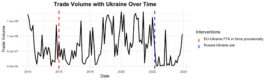
Figures 4.2 and 4.3 provide a closer look at these trends using monthly data. The analysis can be broken down into three distinct phases:

• Phase 1 (2014-2016, before FTA is in force): exhibits a declining trend, potentially reflecting the pre-FTA trade environment and challenges faced by Ukraine during this period.

• Phase 2 (2016-2022, FTA is in force and before the war): shows a slight upward trend, likely indicating a positive response to the FTA, as the agreement facilitated smoother trade flows.

• Phase 3 (2022-2023, FTA is in force and war is ongoing): demonstrates a significant trend shift, marked by an immediate and sudden drop, followed by stagnation. This could reflect the severe disruptions caused by the ongoing conflict between Russia and Ukraine, which has severely impacted trade logistics and economic stability.

While these preliminary findings suggest a relationship between these interventions and fluctuations, it is important to validate these observations through a more rigorous statistical analysis.

The following subsections will discuss preliminary findings for each trade shocks. Additionally, Section 4.2 will delve deeper into these trends using the Seasonal Autoregressive Integrated Moving Average (SARIMA) model, which will allow us to account for seasonality, autocorrelation and other factors that may influence trade patterns. This approach will help confirm whether the trends observed in this exploratory analysis are statistically significant and can be attributed to the interventions, or if they are driven by other underlying factors.

UK-Canada FTA

Unlike the decline observed in Ukraine’s cereals and grains trade post-2022, Canada’s trade in these commodities with the UK shows a different pattern. As seen in Figure 4.4, the trade in cereals and grains has been growing slowly in most years.

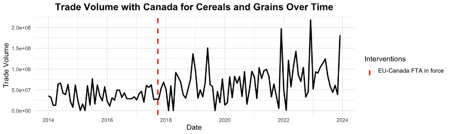
A closer look at the monthly trade volume for cereals and grains in Figure 4.5 reveals two distinct phases:

• Pre-FTA: the trend remains stagnant, with no significant growth.

• Post-FTA: there is a noticeable, albeit slow, upward trend, with new highs that surpass the highest volumes recorded before the FTA.

Spain drought

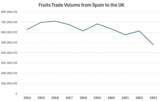
Spain is the UK’s largest supplier of fruits, accounting for 13.5% of the UK’s fruit imports in 2023, according to Comtrade data. However, as depicted in Figure 4.6, the annual imports of fruits from Spain have been slowly decreasing. At the same time, the monthly data in Figure 4.7 shows the following:

• Before the drought: the trend remains stagnant.

• During the drought: there is no significant change in the trend.

• After the drought: the trend remains stagnant for a while, but it begins to slowly decrease, reaching a new low at the end of 2021.

Further statistical analysis to validate these observations is needed, and can be found in Section 4.2.

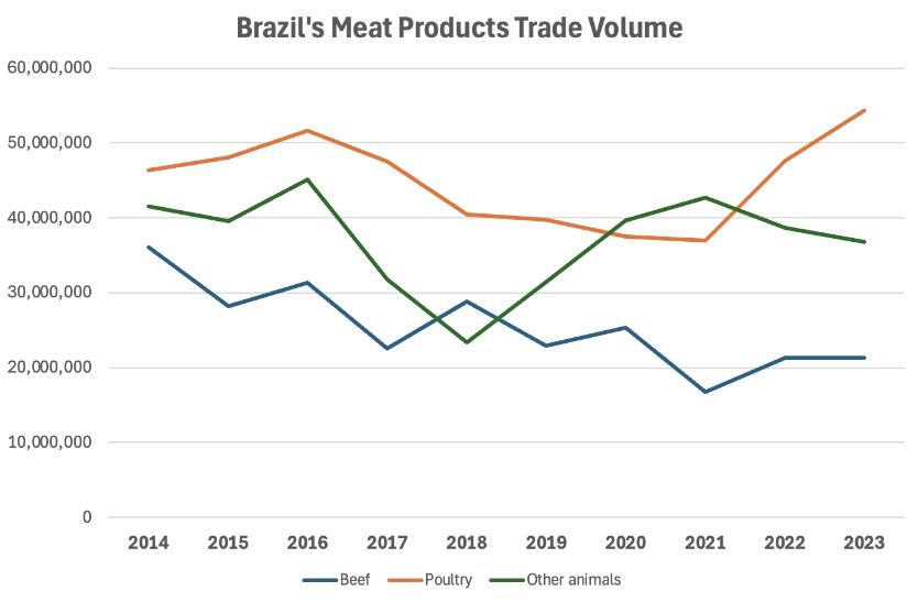
Brazil drought

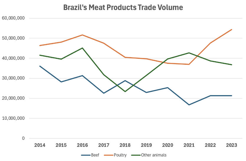
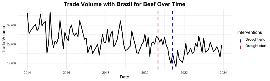
Based on Comtrade data from the FSA, 7.4% of beef imports in the UK come from Brazil. As observed in Figure 4.8, while trade volumes for ‘Other animals’ are stagnating and trade volumes for ‘Poultry’ are slowly growing, trade volumes for ‘Beef’ are declining.

A closer examination of Brazil’s monthly beef trade volume to the UK, shown in Figure 4.9, reveals that while beef trade was already slowly declining before the drought, there was a noticeable dip in beef trade volume during the drought. Importantly, the trade volume has not recovered even after the drought ended.

4.2. Model analysis and discussions

This section continues the analysis from the previous section, presenting and discussing the proposed SARIMA model for each trade shock.

4.2.1. UK-Ukraine FTA

The UK–Ukraine trade is modelled using an ARIMA(2, 0, 0)(1, 0, 0)[12] with two interventions: the FTA and the conflict. Box-Cox transformation is also applied to stabilise the variance of the time series data.

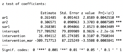
Derived from Figure 4.10, the model can be represented as:

$$\begin{align}Y_{t} =& 717.7093 + 0.2615Y_{t - 1} + 0.3066Y_{t - 2} + 0.2683Y_{t - 12} + 26.4941 \\& \times {Intervention}_{FTA} - 309.7177 \times {Intervention}_{war} + \epsilon_{t}\end{align}\tag{4.1}$$

where:

• $Y_{t}$ = Box-Cox transformed trade volume at time $t$.

• $Y_{t - 1}$ and $Y_{t - 2}$ = autoregressive terms of $Y_{t}$.

• $Y_{t - 12}$ = seasonal autoregressive term capturing seasonality with 12-month lag.

• ${Intervention}_{FTA}$ and ${Intervention}_{war}$ = dummy variables representing the impact of the FTA and the war.

• $\epsilon_{t}$ = error term at time $t$.

Combining Equation 4.1 and Figure 4.11, the coefficients of the interventions can be interpreted as follow:

• {Intervention}_{FTA}: when the FTA is in effect, the Box-Cox transformed trade volume increases by approximately 26.5 units, compared to when the FTA is not in effect. However, since the p-value (0.7560344) for this coefficient is not statistically significant, we cannot confidently say that the FTA has a significant impact on the trade volume.

• ${Intervention}_{war}$ when the war is occurring, the Box-Cox transformed trade volume decreases by approximately 309.7 units, compared to when the war is not occurring. The p-value for this coefficient is 0.0003841, which is statistically significant. This indicates that the war has a significant and substantial negative impact on the trade volume.

While back-transformation process from the Box-Cox scale to the original scale is possible, it requires taking negative values due to the negative coefficient of ${Intervention}_{war}$ which makes the operation invalid. Thus, it is more straightforward to model the original data against fitted value, as shown in Figure 4.12.

As seen in Figure 4.12, the model appears to fit the data reasonably well, with the fitted line closely tracking the original data throughout the entire period. The confidence intervals are relatively wide before the Russia–Ukraine conflict, but overall, the model captures the general trend and seasonal patterns in the data, except for the period after 2022. This might be due to the limited data available, as there are less than two years’ worth of data after 2022, which translates to fewer than 24 data points.

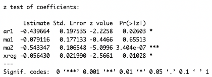
The same analysis is being done for cereals and grains data, modelled using an ARIMA(4, 0, 0)(1, 0, 0)[12] with Box-Cox transformation. The model can be represented as:

$$\begin{align}Y_{t} =& 139.0661 + 0.3196Y_{t - 1} + 0.3142Y_{t - 2} - 0.1303Y_{t - 3} - 0.1790Y_{t - 4} \\&+ 0.2050Y_{t - 12} + 6.7200 \times {Intervention}_{FTA} - 76.4855 \\& \times {Intervention}_{war}\end{align}\tag{4.2}$$

where:

• $Y_{t}$ = Box-Cox transformed trade volume at time t.

• $Y_{t - 1}$, $Y_{t - 2}$, $Y_{t - 3}$, $Y_{t - 4}$ = autoregressive terms of Yt.

• $Y_{t - 12}$ = seasonal autoregressive term capturing seasonality with 12-month lag.

• ${Intervention}_{FTA}$ and ${Intervention}_{war}$ = dummy variables representing the impact of the FTA and the war.

• $\epsilon_{t}$ = error term at time $t$.

Similarly, with Ukraine’s cereals and grains model, the coefficient of ${Intervention}_{FTA}$ is not statistically significant (p-value = 0.6773811), while the coefficient of ${Intervention}_{war}$ is statistically significant (p-value = 0.000003681). This also indicates that FTA is not seen as a significant impact, while the conflict has a substantial effect on trade volume.

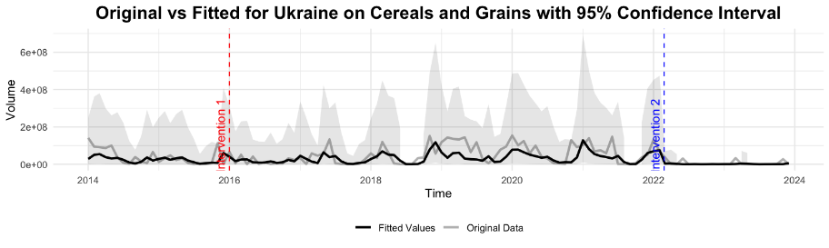
The model is fitted to the original data, as shown in Figure 4.13. While the overall fit is good and the fitted values lie within the 95% confidence interval, the model appears to lack sensitivity after the second intervention, as indicated by its failure to capture three small peaks in the original data. Additionally, the 95% confidence interval is considerably wide, possibly due to the high volatility of the data. This behavior is quite similar to the fitted model in Figure 4.12.

Note that upon conducting the analysis, none of the model assumptions (residuals, stationarity, homoskedasticity or autocorrelation) are violated. As such, these models are good representation of Ukraine’s trade data.

The next subsections will delve into a similar analysis for other trade shocks, allowing for a comparative assessment of different types of trade disruptions.

4.2.2 UK-Canada FTA

The UK–Canada trade in cereals and grains is modelled using an ARIMA(5,0,0)(1,0,1)[12] on its first-differenced data. First-differencing is required to ensure the stationarity of the data. The model, as shown in Figure 4.14, is mathematically expressed as:

$$\begin{align}\mathrm{\Delta}X_{t} =& \ - 0.9805\mathrm{\Delta}X_{t - 1} - 0.6713\mathrm{\Delta}X_{t - 2} - 0.5511\mathrm{\Delta}X_{t - 3} - 0.4973\mathrm{\Delta}X_{t - 4} \\&- 0.3323\mathrm{\Delta}X_{t - 5} + 0.8858\mathrm{\Delta}X_{t - 12} - 0.4730\epsilon_{t - 12} + 534619.7 \\& \times {Intervention}_{FTA}\end{align}\tag{4.3}$$

where:

• $\mathrm{\Delta}X_{t}$ = first-differenced trade volume at time t.

• $\mathrm{\Delta}X_{t - 1}$, $\mathrm{\Delta}X_{t - 2}$, $\mathrm{\Delta}X_{t - 3}$ , $\mathrm{\Delta}X_{t - 4}$ , $\mathrm{\Delta}X_{t - 5}$ = autoregressive terms of $\mathrm{\Delta}X_{t}$.

• $\mathrm{\Delta}X_{t - 12}$ = seasonal autoregressive term capturing seasonality with 12-month lag.

• ${Intervention}_{FTA}$ = dummy variables representing the impact of the FTA.

• $\epsilon_{t}$ = error term at time $t$.

• $\epsilon_{t - 12}$ = seasonal moving average term capturing seasonality with 12-month lag.

The coefficient of ${Intervention}_{FTA}$ is not statistically significant (p-value = 0.7260593). Moreover, this coefficient has a high standard error, indicating that while there is a positive relationship between the intervention and trade volume, the uncertainty around this estimate is substantial.

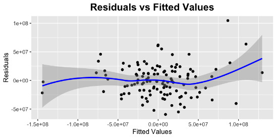
The model complies with stationarity, and the residuals are neither autocorrelated nor normally distributed. However, there is evidence of heteroscedasticity, as indicated by the Breusch-Pagan (BP) statistic of 6.0132 (p-value = 0.0142). Further analysis is conducted using the residuals against fitted plot, presented in Figure 4.15.

Based on Figure 4.15, heteroscedasticity is evident, particularly on the right-hand side, where the spread of residuals increases with fitted values. However, the pattern is not extremely pronounced or dramatic. The curvature of the smoothed line suggests some non-linearity, but the overall distribution is not wildly erratic. While the presence of heteroscedasticity is noted, its impact on the model’s estimates may not be overly detrimental, indicating that the issue is not severe. The primary concern is that the standard errors might be slightly underestimated, potentially leading to overly optimistic confidence intervals and significance tests.

The model is fitted with the original data in Figure 4.16. While the overall trends between the fitted and original data are similar, the fitted values tend to underestimate the trade volumes during peak volumes in the original data. This underestimation could be seen as advantageous from a policymaking perspective. By recognising these discrepancies, policymakers can better plan for food security by ensuring that any shortfalls in cereal and grain imports from Canada are offset by securing additional supplies from other countries. This proactive approach helps mitigate potential risks associated with underestimating import volumes during critical periods. However, at the same time, the model fails to capture the volatility of the data. This is something that requires further study, and that with more data available, this model can mimic the volatility better.

However, based on Figure 4.16, the model also fails to capture the volatility of the data, which is expected given that it does not meet the heteroscedasticity assumption. This unfitness suggests that the model might not adequately account for variations in volatility across different levels of trade volumes. Addressing this issue requires further study, and with more data available, the model could better replicate both the volatility and overall patterns in the data.

4.2.3. Spain Drought

The trade of fruits from Spain to the UK is modelled using an ARIMA(2,0,2)(1,1,2)[12] on its first-differenced data. The model is shown in Figure 4.17 and can be expressed as:

$$\begin{align}\mathrm{\Delta}X_{t} =& \ - 0.2991\mathrm{\Delta}X_{t - 1} + 0.4141\mathrm{\Delta}X_{t - 2} + 0.0247\epsilon_{t - 1} - 0.9044\epsilon_{t - 2} \\&+ 0.7115\mathrm{\Delta}X_{t - 12} - 1.4740\epsilon_{t - 12} + 0.6982\epsilon_{t - 24} - 140526.1 \\& \times {Intervention}_{weather}\end{align}\tag{4.4}$$

where:

• $\mathrm{\Delta}X_{t}$ = first-differenced trade volume at time $t$.

• $\mathrm{\Delta}X_{t - 1}$, $\mathrm{\Delta}X_{t - 2}$ = autoregressive terms of $\mathrm{\Delta}X_{t}$.

• $\mathrm{\Delta}X_{t - 12}$ = seasonal autoregressive term capturing seasonality with 12-month lag.

• ${Intervention}_{weather}$ = dummy variables representing the impact of a weather event.

• $\epsilon_{t}$ = error term at time $t$.

• $\epsilon_{t - 12}, \epsilon_{t - 24}$ = seasonal moving average term capturing seasonality with 12- and 24-month lag.

The large standard error of the dummy variable ${Intervention}_{weather}$, which is 308391.1, suggests uncertainty in its estimate. This leads to failing to reject the null hypothesis for the coefficient of the dummy variable (p-value = 0.648624), rendering it insignificant.

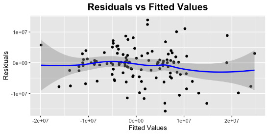
The model meets the requirements for stationarity, autocorrelation, normality of residuals and homoscedasticity. Plotting the residuals against fitted plot shown in Figure 4.18, the residuals appear to be somewhat randomly scattered around zero, which is a positive sign. This is indicative of homoscedasticity, with the BP statistic reaching 1.1066 and a p-value of 0.2928.

Further transformation to ensure that the model fully complies with the model assumptions is possible, but this may result in increased complexity, leading to a lack of interpretability, which is crucial in our case. Therefore, the current model is adequate for proceeding with fitting the model to the original data. Figure 4.19 compares the original data with the fitted model, showing that the current model adequately represents the trade data, especially during the first few years before 2019, or when the drought ended.

4.2.4. Brazil drought

The trade of beef from Brazil to the UK is modelled using an ARIMA(1,0,2) on its first-differenced, log-transformed data. An interesting observation is that the best-fitting model does not account for seasonality lags, unlike the other models considered. This lack of seasonal components makes the model relatively simple and focused purely on autoregressive and moving average terms.

Based on Figure 4.20, the model can be mathematically written as:

$$\begin{align}\mathrm{\Delta}X_{t} =& \ - 0.4397\mathrm{\Delta}X_{t - 1} - 0.0791\epsilon_{t - 1} - 0.5433\epsilon_{t - 2} - 0.0564 \\& \times {Intervention}_{weather}\end{align}\tag{4.5}$$

where:

• $\mathrm{\Delta}X_{t}$ = first-differenced trade volume at time $t$.

• $\mathrm{\Delta}X_{t - 1}$ = autoregressive terms of $\mathrm{\Delta}X_{t}$.

• ${Intervention}_{weather}$ = dummy variables representing the impact of a weather event.

• $\epsilon_{t}$ = error term at time $t$.

Moreover, the model not only complies with key assumptions regarding stationarity, autocorrelation and normally distributed residuals, but also indicates that the weather intervention is statistically significant. As shown in Figure 4.21, the p-value of the coefficient for ${Intervention}_{weather}$ is 0.01028, making it significant at the 5% level. This raises questions about what distinguishes this model from others, particularly since the only other intervention considered statistically significant at the 5% level is the coefficient of ${Intervention}_{weather}$ in the UK-Ukraine model.

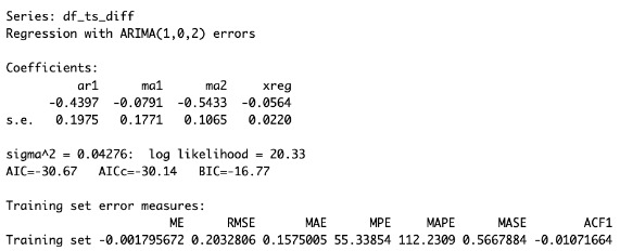
The model was then fitted to the original data to compare the fitted values with the actual data. As shown in Figure 4.22, the fitted values closely track the original data, especially after the drought period, where it tends to slightly underestimate the trade volume. This conservative estimation strategy can be advantageous, as it anticipates worst-case scenarios. Additionally, the 95% confidence interval provides a measure of uncertainty in the model’s predictions, which narrows over time. This suggests that the model’s predictions become more reliable as more data becomes available, making it a valuable tool for forecasting future trade volumes.

5. Conclusion and Recommendation

This chapter concludes the study and is divided into two sections. The first section summarises the findings from each of the four models. The second proposes recommendations for future research in this area based in the insights gained from this study.

5.1. Conclusion

This study explored the impact of free trade agreements (FTAs) and weather-related events on the United Kingdom’s (UK) food and feed commodity imports. The analysis focused on the UK’s trade agreements with Ukraine and Canada, as well as the effects of significant droughts in Spain and Brazil. By applying the Interrupted Time Series (ITS) methodology in combination with the Seasonal Autoregressive Integrated Moving Average (SARIMA) model, we were able to quantitatively assess the effects of these shocks on trade volumes by creating appropriate SARIMA models for each case.

After a thorough analysis, the findings revealed the following:

• The UK–Ukraine FTA showed no statistically significant impact on the trade volumes of cereals and grains from Ukraine. However, the ongoing conflict between Russia and Ukraine had a substantial and significant negative effect on these trade volumes, underscoring the profound impact of geopolitical instability on international trade.

• The UK–Canada FTA did not exhibit a statistically significant impact on the trade volumes of cereals and grains from Canada. However, visual inspection of the data suggested a potential upward trend in trade volumes following the FTA. This discrepancy indicates that while the statistical analysis did not confirm a significant effect, there may be underlying factors or market dynamics contributing to the observed increase in trade volumes. Further investigation could explore these aspects in more detail.

• Weather-related trade shocks, specifically the droughts in Spain and Brazil, had varying effects. The drought in Spain did not significantly impact the UK’s import of fruits, indicating resilience or the presence of alternative sources of supply. In contrast, the drought in Brazil led to a significant and lasting decrease in beef exports to the UK, highlighting the vulnerability of specific commodities to extreme weather events.

The results of this study are mixed, making it difficult to generalise whether FTAs and weather events consistently impact trade volumes. However, when considering each case individually, the study conclusively demonstrates that the conflict in Ukraine significantly and negatively affected Ukraine’s cereal and grain exports to the UK, and the drought in Brazil had a marked adverse effect on beef imports from Brazil to the UK.

Despite the practicality of the SARIMA model, which is simpler compared to other related works that require multiple variables and more extensive datasets, this approach also comes with several limitations, including:

1. Omission of complex interactions: the simplicity of the SARIMA model may lead to the omission of interactions between multiple variables that could significantly influence trade volumes. This could result in an incomplete understanding of the factors driving changes in trade.

2. Stringent model assumptions: the ITS model assumes that only the specified interventions, represented by dummy variables, are influencing trade volumes. This assumption is stringent and does not account for other simultaneous disruptions or external factors that may impact trade dynamics. Furthermore, the SARIMA model itself relies on several strict assumptions, such as the requirements for stationarity, linearity, and independence of residuals. These assumptions may not fully capture the complexity and variability inherent in real-world trade data, potentially leading to biased or inaccurate results if they are violated.

3. Subjective definition of disruptions: the definition of what constitutes a disruption can be subjective. Without standardised criteria for identifying and categorising these events, there may be inconsistencies in how different disruptions are interpreted and analysed, potentially affecting the reliability of the conclusions.

4. Data availability: the completeness of the data is crucial for reliable results. This study is limited to 10 years of data, with each data point representing a month. This limits the study to 120 data points for each model. Additionally, the availability of enough data points before, during, and after the intervention must be considered. For example, the UK-Ukraine FTA model has only 22 data points for the dummy variable representing the Russia-Ukraine conflict. This raises the question of whether 22 data points are sufficient to demonstrate statistical significance, and whether the results would still be statistically significant at the 5% level if the number of data points were different. Furthermore, the 2014 Russian invasion of Crimea, part of Ukraine, was not captured in the model due to the limited data available prior to 2014 (Kofman et al., 2017).

5. Generalisation of the results: The findings are based on specific cases involving the UK and its trade partners. As such, the results may not be easily generalisable to other contexts, regions, or commodities, limiting the broader applicability of the study.

6. External factors: The focus on FTAs and weather events means that other external factors, such as global economic trends or technological advancements, may not be fully accounted for. These factors could also drive changes in trade volumes, which means that this study may oversimplify the trade environment.

Therefore, while the model provides valuable insights, caution must be exercised when interpreting the results. The findings should be considered within the context of the study’s limitations, particularly the potential oversimplification of complex trade dynamics and the challenges of modelling in the face of highly volatile geopolitical and environmental factors.

5.2. Recommendation

Based on the findings and limitations of this study, several recommendations are proposed for future research. To improve the accuracy and reliability of future analyses, it is crucial to expand the scope of trade data. This includes ensuring that the data encompasses a longer historical time period, providing more extensive insights into trends and enabling more robust analyses. With more comprehensive data, the standard error of the estimates may be reduced, potentially affecting the statistical significance of the coefficients and yielding more precise and reliable results.

To further validate the findings and enhance generalisability, it is recommended to test this methodology on other trade datasets. By applying the same analytical framework to different datasets, researchers can assess how the results vary on a case-by-case basis and determine the robustness of the methodology across different trade relationships and commodities.

Standardising the criteria for defining and identifying trade disruptions is also recommended to enhance the consistency and reliability of studies in this area. While this study primarily focused on FTAs and weather events, it is important to explore the impact of other trade shocks, such as health crises and supply chain disruptions, on trade volumes. Additionally, employing more advanced modelling techniques that can better handle non-linearity and structural breaks in the data may capture more intricate trade dynamics and improve predictive accuracy.

From a policy perspective, the significant impact of geopolitical events, such as the Russia-Ukraine conflict, highlights the need for robust contingency plans and strategies aimed at diversifying trade partnerships and strengthening domestic production capabilities. Continuous monitoring of trade flows, coupled with adaptive strategies that allow for quick responses to emerging challenges, will be essential in mitigating the negative impacts of unforeseen events. By addressing these areas, future research can build on the findings of this study, while policymakers can be better equipped to navigate the complexities of global trade, ensuring greater stability and resilience.

---

1. https://www.food.gov.uk/research/research-projects/list-of-commodity-codes-and-categories

2. https://www.uktradeinfo.com/

3. https://cran.r-project.org/web/packages/readxl/index.html

4. https://cran.r-project.org/web/packages/lubridate/index.html

5. https://cran.r-project.org/web/packages/forecast/index.html

6. https://cran.r-project.org/web/packages/tseries/index.html

7. https://cran.r-project.org/web/packages/lmtest/index.html

8. https://cran.r-project.org/web/packages/ggplot2/index.html

9. https://cran.r-project.org/web/packages/gridExtra/index.html

10. https://cran.r-project.org/web/packages/MASS/index.html